So far on our algorithmic trading journey we have only looked at technical analysis. Essentially, we have been treating price as a time varying signal whose future movements can be forecast by examining past movements. Today, we will take a look at the Price-to-Earnings Ratio. I will start with looking at what the P/E ratio is, then I will show the statistical properties of the P/E ratio for the S&P 500, and finally, I will show the relationship between 1-year returns and the P/E ratio.

Disclaimer

I am not licensed as a financial advisor by IIROC. The information provided on this website does not constitute investment advice, financial advice, trading advice, or any other sort of advice. Conduct your own due diligence before making any life altering or investment decisions.

1. What is P/E?

The Price-to-Earnings ratio is calculated by taking the price of a security and dividing by its last 12 months of earnings. The P/E ratio is the answer to the question of: ‘how much are investors willing to pay for $1 of current earnings?’. In general, if earnings are negative the P/E ratio is treated as ‘undefined’.

A high P/E ratio can be an indication that investors expect high earnings growth-they are willing to pay a high price for current earnings in exchange for substantial future growth. If that growth does not materialize investment returns can suffer. A low P/E on the other hand should indicate high future returns-investors are paying a low multiple of earnings and hence earn back their investment more quickly.

To get a better sense of what constitute high and low P/E it can be helpful to make a comparison to historical trends, or in the case of a company to other companies in the same industry.

For now let’s take a look at the P/E ratio for the S&P 500 over the last 20 years.

2. Statistical Properties

Before I dive in here, the data on the historical P/E ratio is from multpl.com.

Let’s start with some exploratory data analysis:

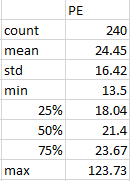
Over the last 20 years the P/E ratio has looked like this:

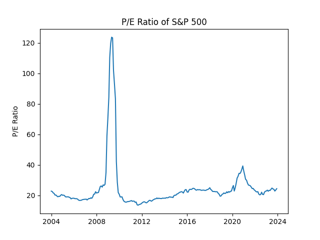
The mean P/E over this time was 24.45 with a standard deviation of 16.42. There were notable excursions from the mean in 2009 and 2020. In 2009 the P/E was over 100, and in 2020 the P/E reached 40. In both cases there were significant declines in earnings as a result of the subprime crisis and the COVID-19 pandemic. Earnings appear in the denominator; small values can quickly send the ratio shooting off towards infinity.

The distribution looks something like this:

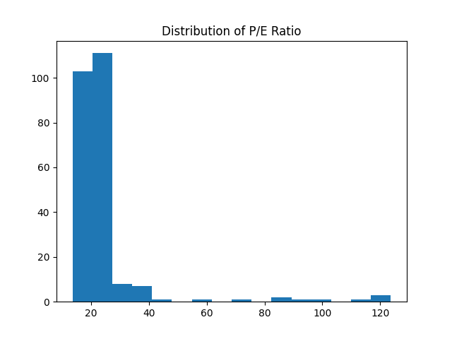
The distribution is heavily skewed to the right-the mean is just above the 75^th percentile and there is a long tail of large outliers. The outliers are going to cause some problems in the next section.

3. Relationship between Return & P/E

We will use a linear regression to determine the relationship between 1-year forward returns and P/E. One of the key assumptions in linear regression is that our data be (roughly) normally distributed. The P/E data is much too skewed for the regression to be valid. The fit looks like this:

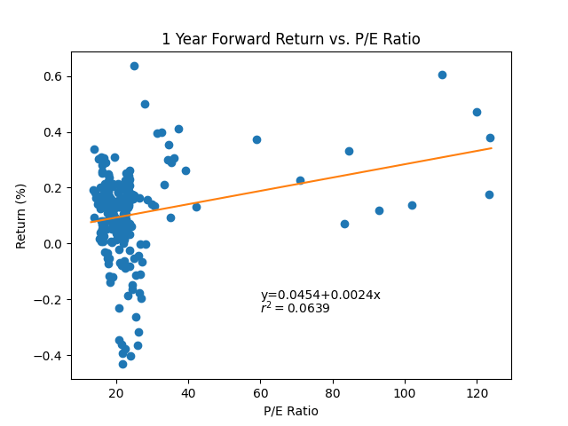
The equation is telling us that for every 1 unit increase in P/E we should expect and additional 0.2% annual return. The result does not match our intuition that low P/E ratios should be associated with high returns. Those outliers are having an outsized impact on our model.

If we eliminate the outliers and only consider P/E ratios less than 30 the distribution becomes much less skewed:

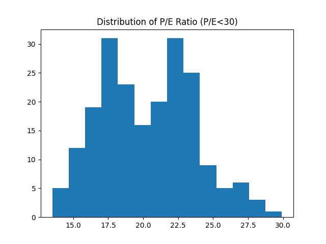
This distribution is bi-modal but it is much closer to a normal distribution, and at the very least is symmetric.

If we regress return against P/E we get a relationship that now looks like:

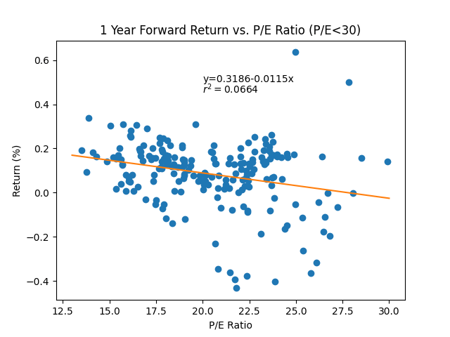
Now the equation better matches with our intuition. For every 1 unit increase in the P/E ratio we should be expecting annual returns to decline by 1.15%. The relationship is not particularly strong; the co-efficient of determination (r²) is only 0.0664 – only 6.64% of the variation in 1 year returns is explained by variation in the P/E ratio.

Before leaving this topic, let’s check to see if the slope differs significantly from zero. We will conduct a t-test with hypotheses (H₀: β₁ = 0, H₁: β₁ ≠ 0). To do this we will look at the analysis of variance (ANOVA). The ANOVA table is shown below:

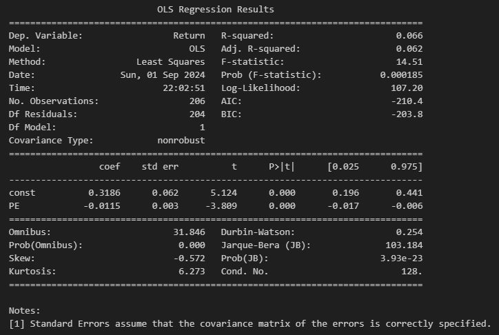
To determine whether the measured slope differs significantly from zero we need to look at the F-statistic. The F-statistic is well within the rejection region (P<0.05): we can reject the null hypothesis that β₁ = 0 in favour of the alternative hypothesis β₁ ≠ 0

4. Conclusion

The above analysis showed that there is a relationship between the Price-to-Earnings ratio and one year forward returns. The relationship is weak and there are many (unknown) factors that were excluded from the analysis. I will continue to develop this analysis in future posts, so, as always, stay tuned!