The next step (long overdue) on our algorithmic trading journey is a dive into gradient methods. In a previous post I looked at optimizing the parameters of a moving average trade signal by brute force – visiting all possible combinations of short term and long term moving averages. Brute force methods are limited to small parameter spaces; recall that the size of the parameter space was reduced by incrementing the moving average period by five, and in any case brute force methods lack elegance.

This post is intended to be a primer; I plan to use gradient methods in future posts on optimizing trading methods, so the usual disclaimer applies.

Disclaimer

I am not licensed as a financial advisor by IIROC. The information provided on this website does not constitute investment advice, financial advice, trading advice, or any other sort of advice. Conduct your own due diligence before making any life altering or investment decisions.

1. Gradient Descent in General

A common problem in machine learning is finding the extreme values (maximum or minimum) of a function. For example in Linear Regression (more on this in a future post) we seek to minimize the mean squared error between estimated values and measured values by choosing the weighting for each independent variable.

Gradient descent works by constantly moving ‘downhill’ to smaller values of an objective function. You can think of it as trying to locate the lowest point in North America (Death Valley) by rolling a soccer ball: it ought to work, but there are a number of practical problems. I will discuss two of them here:

1. Local minima
2. Zero gradient

Local Minima

A local minima is a low point of the function, but not necessarily the lowest point in the domain of interest. Gradient descent can be prone to falling into local minima, and in its basic form, has no way of getting out of the neighbourhood of the minima. Which minima the algorithm converges to is dependent on the starting position.

If I were to start the process of finding the lowest point in North America at my front door in Calgary, I would rather quickly find myself following the Bow River east, and eventually winding up in Hudson’s Bay. While this is lower than where I started (yay!), it is not where I wanted to wind up.

Zero Gradient

The condition for stopping this algorithm is that the gradient of the objective function is equal to zero – this will be true at any extreme value (minimum or maximum) of the function. The gradient gives no information on whether the point reached is a minimum, maximum, or just locally flat. Think of starting our soccer ball in Saskatchewan – no matter which direction we go there is no hill to roll down, and no way to sensibly update our position.

Let’s take a look at examples in one and two dimensions before revisiting the moving average trade signal.

2. Gradient Descent in 1-D

To get a sense of how this works, we will start with a function of a single variable. For this example, I will find the minimum of:

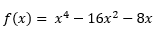
When this is plotted it looks like this:

From an inspection of the graph there are minima at about x=-2.5 (local) and x=3 (global) and a maxima at about x=0 (local – strictly we also need to consider the end points of the domain (x=±4)).

While we could find the minima and maxima by differentiating the function once, and setting that equal to zero then solving for x, that seems like a lot of work (especially for a post about gradient methods).

Instead of doing all that, we will pick a random starting point (x₀) and update our position according to:

We will continue this update process until the change between iterations is ‘small’ – once the term df(x₀)/dx reaches zero we are at either a local minimum or maximum, and in this form of gradient descent we have no way to move off of either of these points.

The term denoted by γ is the learning rate: a parameter that controls the step size. If this is too small the algorithm will take many steps to converge to the minimum; if this is too large the algorithm runs the risk of missing the minimum by stepping back and forth from one side of the valley to the other. Setting γ appropriately can be a bit of a black art – there is a wikipedia article here – but in this case I have simply chosen γ = 0.01.

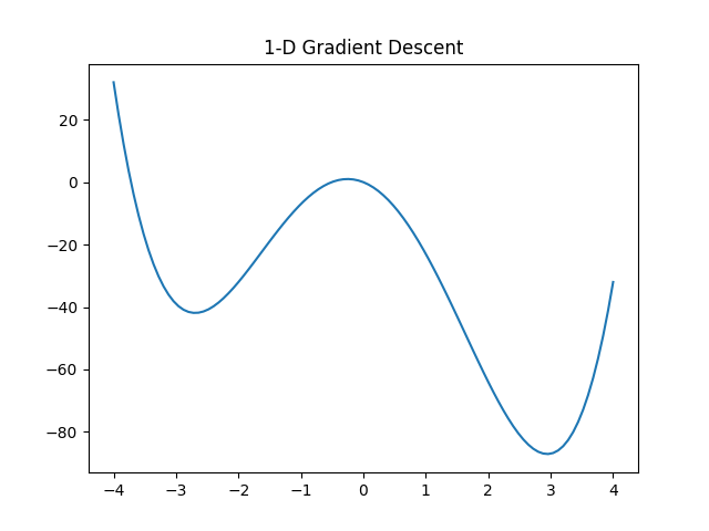
Let’s see what this looks like! I have picked three arbitrary starting points: x=-3.5, -0.252, and 1.5

The first starting point (x=-3.5) finds the local minima. The second starting point (x=-0.252) happened to start at the local maximum (df/dx=0) and could not update its position. The third starting point (x=1.5) finds the global minimum – Success!

This process is not limited to one dimension; it will work in any number of dimensions. Lets take a look at an example in two dimensions.

3. Gradient Descent in 2-D

The process here does not really change all that much, we will just need more subscripts to keep track of which dimension we are talking about. Hopefully that means more pictures and fewer words.

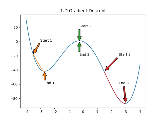
The function we will look at this time is:

For those who find this impenetrable (Hey! Me too!) it looks something like this:

This function has many of the same features as our 1-D example: a local minimum, a global minimum, and some flat spots. I have also plotted the contours below the function.

The function we will use to update our position now looks like:

It is the same thing, just with an extra dimension: a is some point (x,y) on our function. γ is still the learning rate, for this example I have chosen a learning rate of 0.2. ∇ is the vector derivative operator, it works similarly to the 1-D derivative operator – we just have to look in all directions.

Again, I have picked three starting points (-1,-0.5), (3,-3), and (0,2) to illustrate how the method progresses and how it can fail.

It is a bit hard to see, but the path is always perpendicular to the contours – the algorithm finds the direction where the function is the steepest and proceeds in that direction.

The first starting point (-1,-0.5) finds the local minimum. The second starting point (3,-3) starts in a flat spot, and can not update its position. The third starting point (0,2) finds the global minimum – Success!

4. Moving Averages Revisited

Let’s wrap this up by revisiting the post about optimizing a trade signal constructed from the difference between a long term and a short term moving average.

We will take a look at how gradient methods can be used to explore the space, moving from a random point to a ‘better’ point. First, I brute forced the space with an increment of one day – recall in the original post I used an increment of five days to reduce the computational effort. This step is not really required, except for making nice plots, and knowing where the maximum is in case the gradient method fails (spoiler alert). Second, I picked seven random starting points and told my computer to have at it. From its current position , the algorithm looks in all four directions, and computes the return at all four adjacent points, if any of the four surrounding points has a higher return than the return at the current position, the algorithm updates its position to whichever position has the highest return. This process is then repeated until a local maximum is reached.

The assumptions for assessing performance are unchanged from the previous posts:

1. $1000 starting capital
2. No commissions
3. Only whole numbers of shares may be traded
4. No cash is added during the study period
5. Dividends are not considered
6. No short selling

Let’s see what happened!

As it turns out none of the chosen starting points found the global maximum (9,75). The pink path is the closest; I started that one at (12,75) and it ended after taking two steps at (11,74).

Gradient methods are somewhat reliant on the function being smooth; functions in the real world are lumpy and bumpy with lots of local minima/maxima. There are methods that can overcome the tendency to settle at a local optimum, but those will have to wait for a future post – this post has gone on long enough.

5. Conclusion

Gradient methods are a common way to find the extreme values of a function, but are somewhat limited by being myopic-this can lead to them getting stuck at a local extreme and never exploring the space further. There are ways to overcome this, but that will be the subject of a future post – stay tuned!