We will pick up where the previous post left off, and continue our adventure through algorithmic trading by optimizing some of the parameters used by the Moving Average and Kalman Filter signals.

Disclaimer

I am not licensed as a financial advisor by IIROC. The information provided on this website does not constitute investment advice, financial advice, trading advice, or any other sort of advice. Conduct your own due diligence before making any life altering or investment decisions.

1. Optimizing the Moving Average Signal

A question that arises from the previous post is: Was there any method to the madness of selecting the periods (20 & 50 day) used to compute the moving average signal?

Spoiler Alert: There was not

What periods then should be selected to yield the maximum return? And what is the standard deviation of the return we can expect by using those particular periods?

To explore this question, I will let the long term moving average vary between 20 days and 100 days (in 5 day increments), and the short term average vary between 10 days and 50 days (in 5 day increments). Let’s see what happens over the full 20 year period:

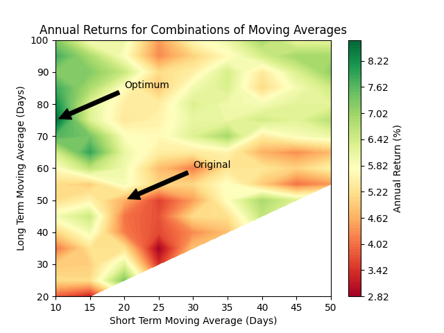
The best performing moving average model was the 10, 75 model: a 10 day short term average combined with a 75 day long term average.

Wow! The annual return for the moving average can be increased by a little over 4% annually just by correctly selecting the periods used for averaging.

The particular method I used for finding the optimum-Brute Force (just visiting all possible combinations of parameters) only works here because the parameter space is small; there are at most 153 possible combinations of moving averages (less where the short term average is longer than the long term average). I will revisit this in the future and explore using a gradient descent to find the optimum – stay tuned!

2. Optimizing the Kalman Filter

The choice of parameters for the Kalman Filter signal (0.01, 0.001) was, like the Moving Average signal, arbitrary. We can do the same thing with the transition co-variances in the Kalman Filter as we did with the periods in the Moving Average. The trouble here is that I don’t have a very good intuition about the ranges these parameters should take on: transition co-variance is somewhat abstract.

My first attempt looked like this:

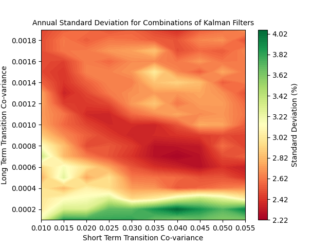
This graph shows that when the short term co-variance approaches zero, the filter performance becomes poor, no matter the long term co-variance. We should look for an optimum filter somewhere in the range of (0.03, 0.001). When we isolate this part of the parameter space (notice the change in scale) it looks like this:

The best performing Kalman Filter had transition co-variances of 0.045 (short) and 0.008 (long).

3. Five Year Performance

As with the previous post, I will assess the performance of each model against a Buy and Hold strategy in five year increments, beginning with July 2004, and incrementing each month until January 2019. The moving average models produced a mean and standard deviation that looked like:

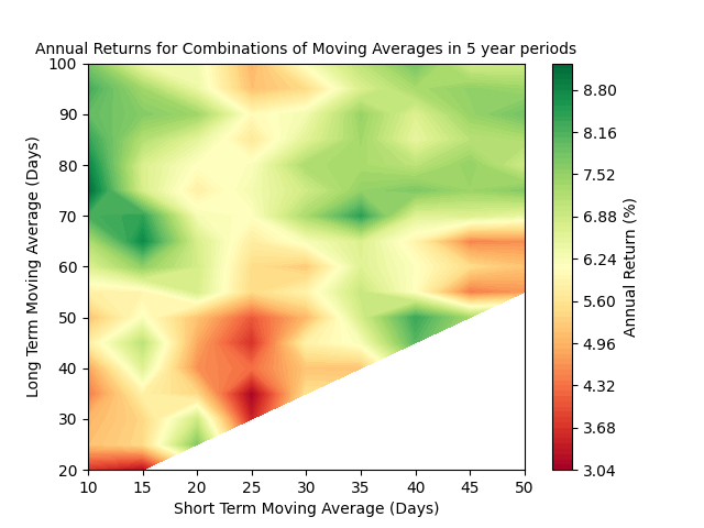
Recall that we would like to minimize the standard deviation, but there is also a positive correlation between return (reward) and standard deviation (risk):

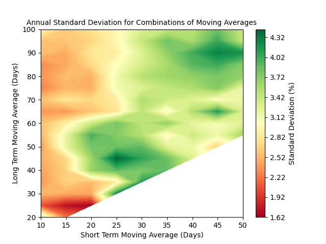
It appears that (by happy accident!) the moving averages that produce the maximum return also produce a low (but not minimum) standard deviation.

The Kalman Filter models produced means and standard deviations that looked like:

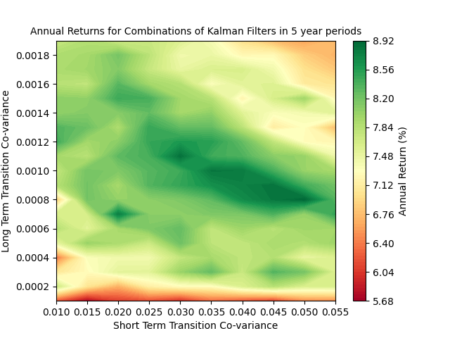
The optimal model did change slightly, the best model here used a short term transition co-variance of 0.05.

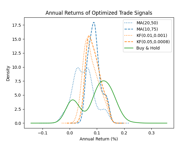
I’ll wrap up by comparing the annual returns from the original model and the optimized models to a Buy and Hold strategy. All of these are taken over five year holding periods, beginning each month starting in July 2004. The original models are shown with dotted lines, the optimized models are shown with dashed lines:

4. Conclusion

Choosing optimal parameters significantly improved the moving average model. The Kalman filter model was not as affected by the choice of parameters, but we were still able to improve the end results.

In a future post I will revisit this optimization, but show how to use Gradient Descent to traverse a path to the optimal parameters without having to map the entire space.